 {width="4.791666666666667in"
height="2.721790244969379in"}
{width="4.791666666666667in"
height="2.721790244969379in"}Classifier: predict a category
Regression: predict a value, continuous quantities
Supervised learning: you know the target value on the learning set. Initial target values generally from human input, crowdsourcing (e.g. Crowdflower) for paid people to classify. Maybe get implicit values from user actions, e.g. happy with search results when don't come back to to a search.
Unsupervised: find structure where no labels known. Clustering, unsupervised outlier detection.
Workflow:
Representation (choose features, type of classifier). Features are columns of the dataframe. Feature extraction.
Evaluation (choose criterion, e.g. % of target variables correctly predicted on test set)
Optimisation (how to get the best parameters, e.g. try a range of K values in Knn).
Score gives matches.
Predict gets values
Sklearn values ending with _ are model derived values from training data.
For maths see Andrew Ngs machine learning course on coursera.
Instance or sample are the rows. Features are the columns. Convention is X for the matrix of data.
Target value is label (classification) or continuous value (regression). Convention is y.
Default split for train / test is 75%
Train test split function returns the partitioning of X, y into X_train, X_test, y_train, y_test.
Model fitting uses the scikit learn estimator to set the parameters for the model. Updates internal state of the model.
Evaluation methods.
Score method
Predict method for new instances.
Binary classification has 2 outputs, normally 0 and 1 (eg credit card fraud). Multi class classification gives more complex classification (e.g. label for fruit, each has only one label). Multi-label classification where there are multiple target values applicable, e.g. classifier for the multiple things that a web page is about with different strengths. Continuous value means regression problem.
Some models have both regression and classification applications e.g. SVM.
Unstable predictions mean that small changes to the training data can produce different predictions.
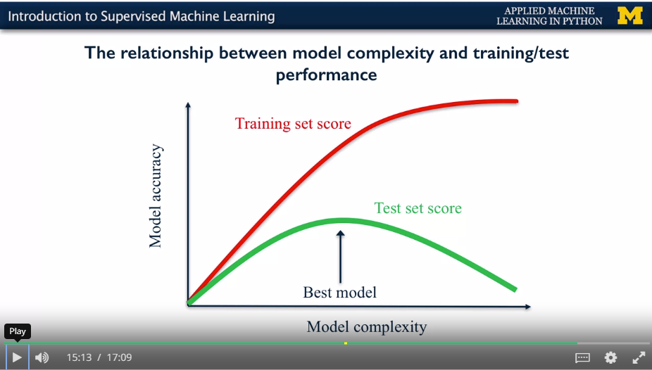
Overfitting: Relationship between model complexity and model accuracy. Overfitting is detrimental to new data predictions.
 {width="4.791666666666667in"
height="2.721790244969379in"}
Model is the mathematical representation which translates the input variables to the output variables.
Language: Independent variables / dependent variables in stats, Features / target values in ML.
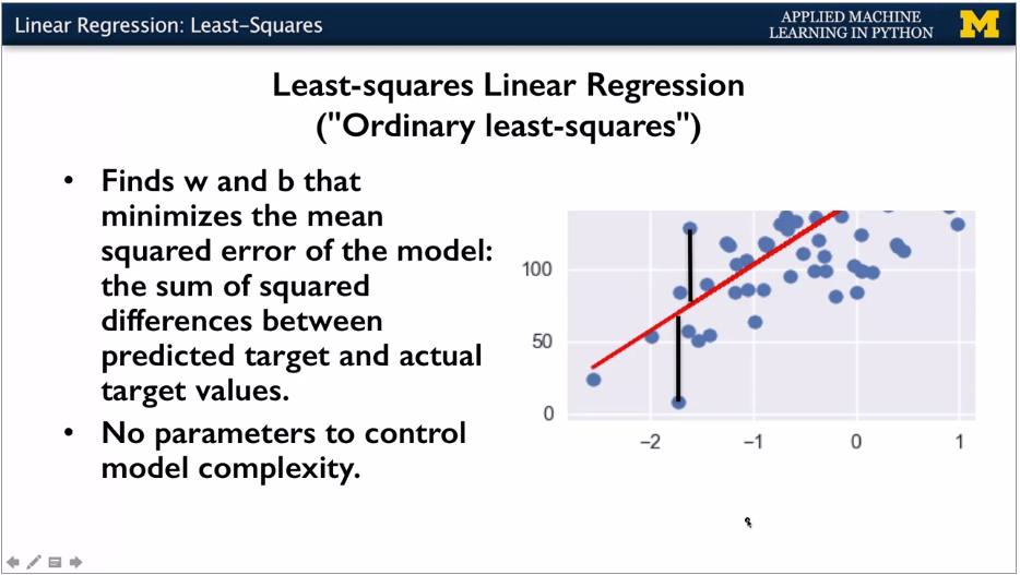
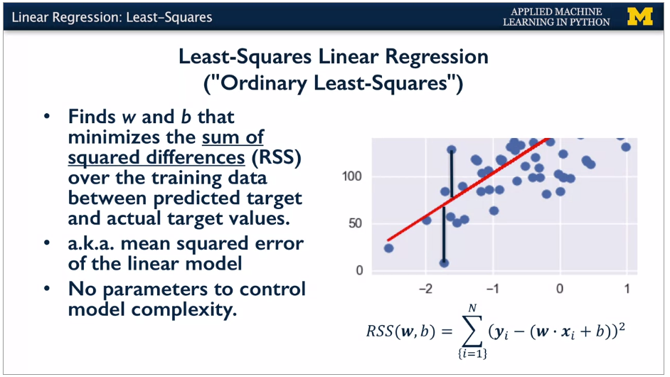
For each training point, take the difference between the predicted y and the known y. Square.
Known as RSS, residual sum of squares. Often this is the objective function being minimized.
 {width="4.707503280839895in"
height="2.65625in"}
 {width="4.726061898512686in"
height="2.65625in"}
 {width="4.706944444444445in"
height="2.6486340769903762in"}
 {width="4.708333333333333in"
height="2.659847987751531in"}
 {width="4.614583333333333in"
height="2.617623578302712in"}
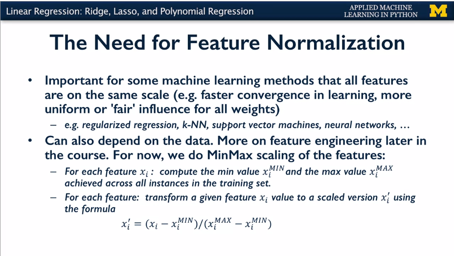
transform input features so all are on the same scale. Necessary when using ridge regression. Feature normalization is generally done.
 {width="4.385416666666667in"
height="2.4764534120734907in"}
get range, get difference between a value and the min, divide by the range. Gets 0 for min, and 1 for max.
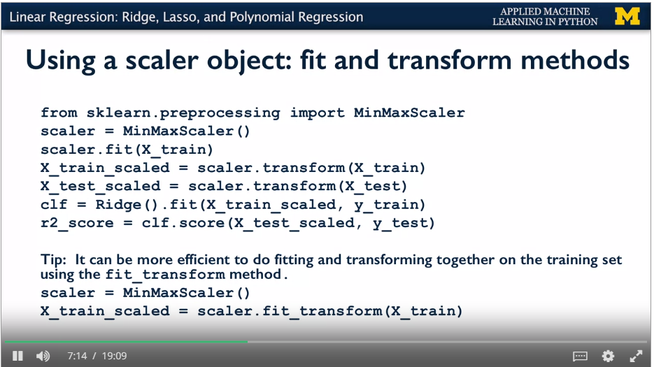
Need to apply the same scaling object to training and test sets. Fit the scaler to the training data only, otherwise get data leakage from the test data to the training data. Model may be harder to interpret after scaling.
 {width="4.479166666666667in"
height="2.515003280839895in"}
Memorise the data -> 100% accuracy.
Generalise well: Ability to perform well on held out test set. Assumption that the future test set is drawn from the same population as the training set.
Inadequate amount of training data means overfitting, and doesn't generalise well.
Underfit: don't match the complexity of the data well. Linear model on a curve.
Overfit: too much memorising, doesn't generalise well. E.g. Highly polynomial for smooth curve. Not enough data to regognise the global trend. Captures too many fluctuations in the training data.
Knn: with a low value of K, get highly granular decision boundaries, so higher risk of overfitting. With high value, doesn't capture enough features.
Data sets with many features are common in real world (high dimensions).
This penalises complexity, reduces overfitting. E.g. the penalty factors in ridge regression.
Knn memorises whole training set, gets the k nearest neighbours for a new point, takes vote of the outcomes. Higher k gives lower model complexity. Can be used on non binary classifiers, and regression. For regression, takes k values nearest to the test point and averages (or other measure e.g. weights) to get target variables. Not good model for large number of features
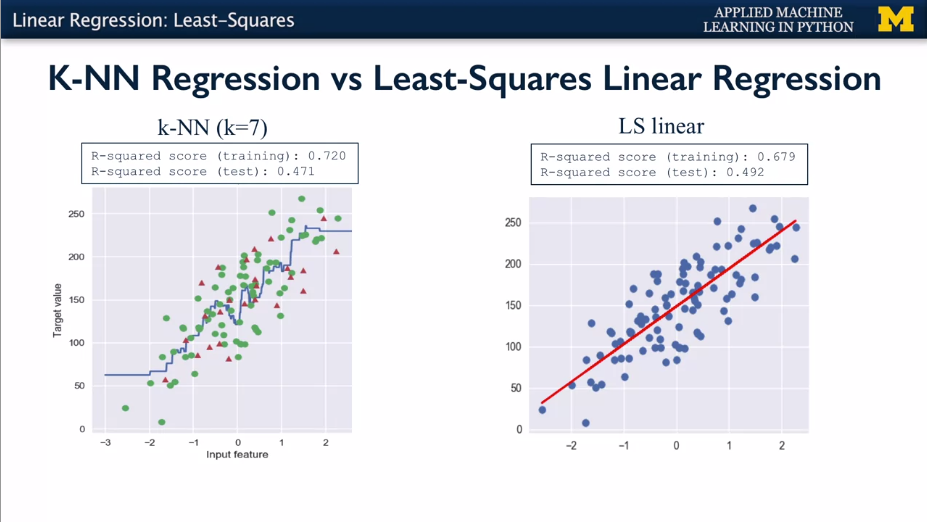
R-squared regression score (also called coefficient of regression) gives 1 for perfect prediction.
Get training set R squared, and test set r squared. Get the graph of model complexity vs model accuracy.
Distance function: Euclidean is default.
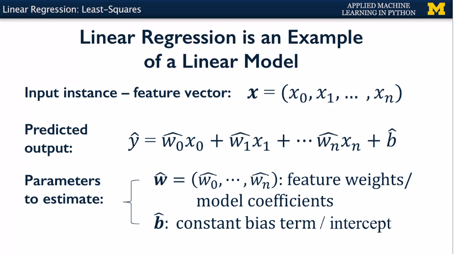
Sum of weighted variables. Training means estimate the parameters for the model to minimise the error. Strong assumption that there's a linear relationship.
B term is y intercept, also called the bias term.
 {width="4.5in"
height="2.509250874890639in"}
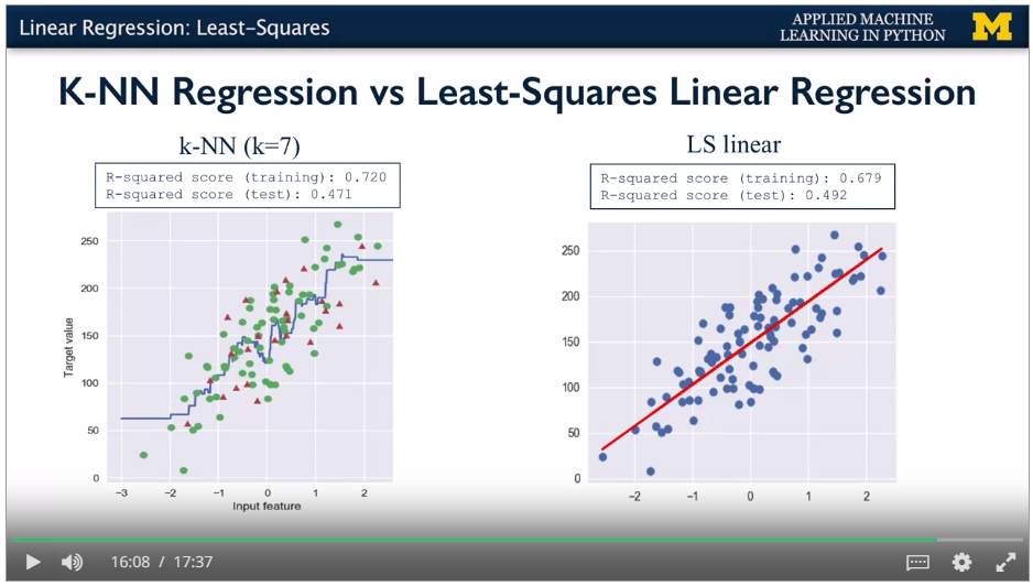
Least squares is square of the difference between the model predicted value and the training points set. Sum of squared differences is RSS (residual sum of squares).
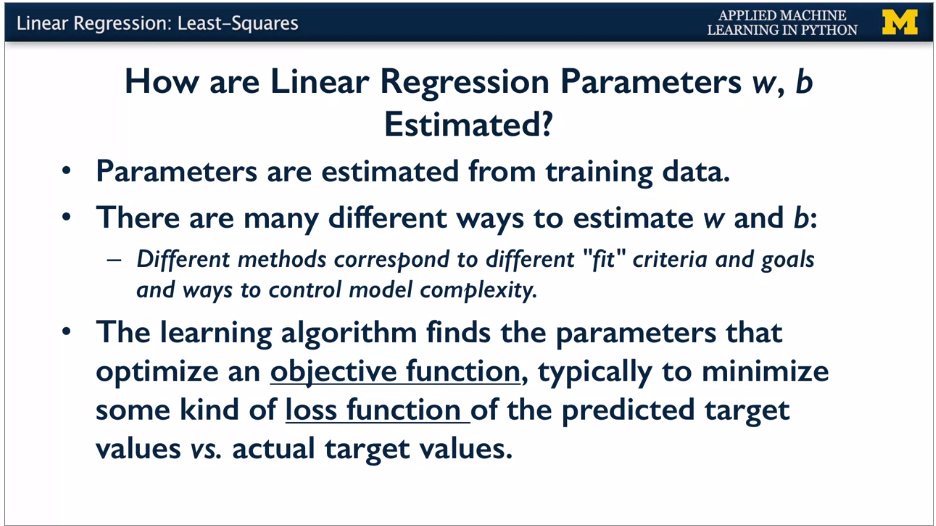
Maximise the objective function. Typically this is some kind of loss function of the predicted target values vs actual target values. Learning algorithm sets the parameters to minimuse the objective function. Simple case this is to minimise the RSS.
No params for model complexity, just a straight line using all training data.
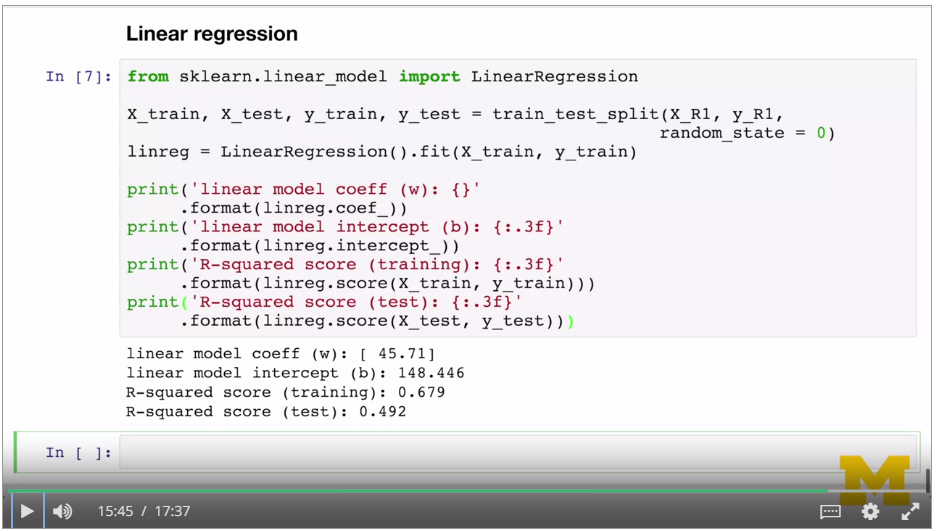
Sklearn.linear_model.LimearRegression. Coefficients are in linreg.coef_ and linreg.intercept_ values.
Use linreg.score to get RSS.
 {width="4.75in"
height="2.67496719160105in"}
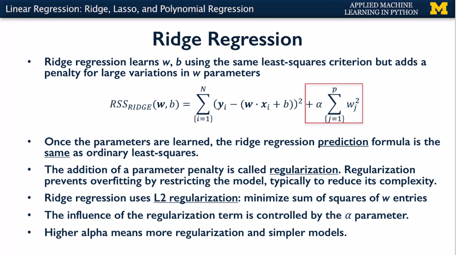
Ridge regression adds a penalty for high weights (w) to the function being optimised. This penalises complexity, reduces overfitting, called Reglularisation. Good when lots of features. Linear_model.Ridge class, and specify alpha parameter. Need to normalise first.
Regularisation is useful when small amounts of training data relative to number of features. Less useful when large amounts of training data. As change alpha, get the usual overfitting vs complexity trade off, with a value of alpha that is a good trade off between complexity and overfitting.
 {width="4.8125in"
height="2.679238845144357in"}
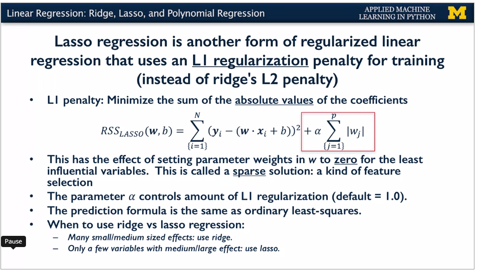
Penalty is L1, sum of the mods of the w's. Model is easier to interpret. Forces unimportant factors to zero. Good when a few features have a large effect. This is a sparse solution, automatically selects features.
 {width="4.856826334208224in"
height="2.7604166666666665in"}
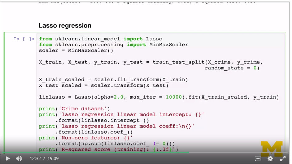
Use lasso:
 {width="4.947916666666667in"
height="2.79080927384077in"}
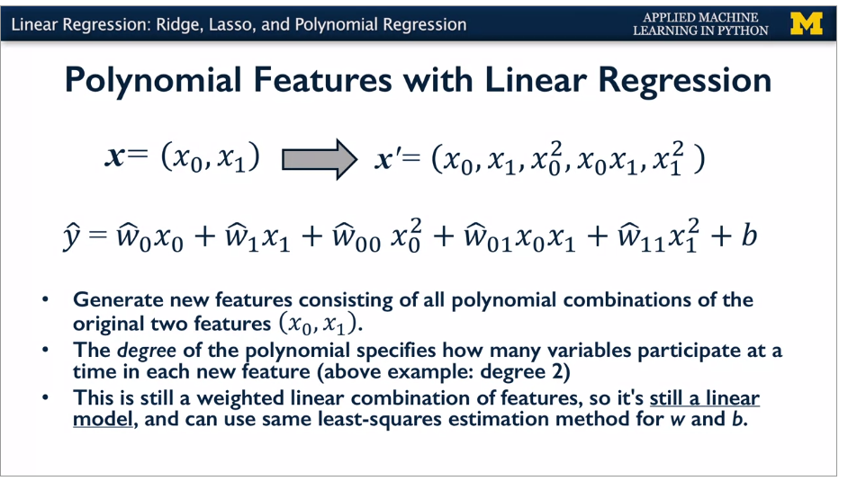
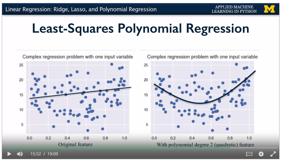
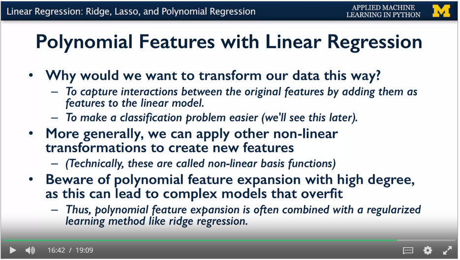
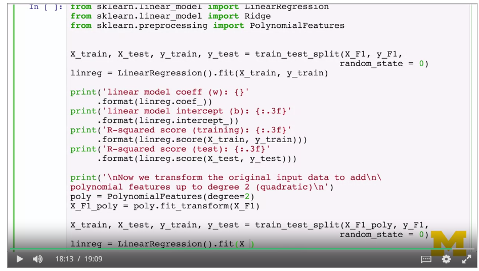
Artificially take combinations of the factors (squares, x~0~x~1~ etc) and get factors for these. Treat as a linear regression, and minimise RSS. Degree of polynomial says the combinations. Still a linear model.
 {width="4.933021653543307in"
height="2.8020833333333335in"}
 {width="4.447916666666667in"
height="2.5526487314085737in"}
 {width="4.5in"
height="2.541159230096238in"}
 {width="4.5in"
height="2.5471412948381453in"}
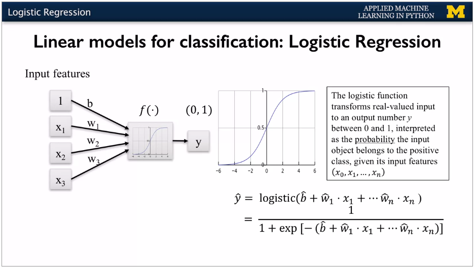
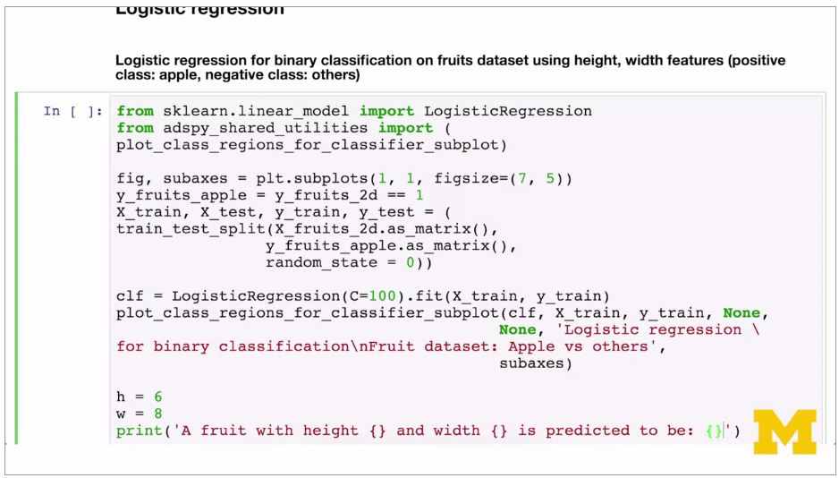
Used to produce a binary outcome, not continuous. Standard linear, but apply the logistic expression to compress the output to a range 0 -> 1. Can also be multi class, non binary. Same as linear but runs it through the sigma function. This compresses the result to 0 or 1.
 {width="4.489583333333333in"
height="2.529805336832896in"}
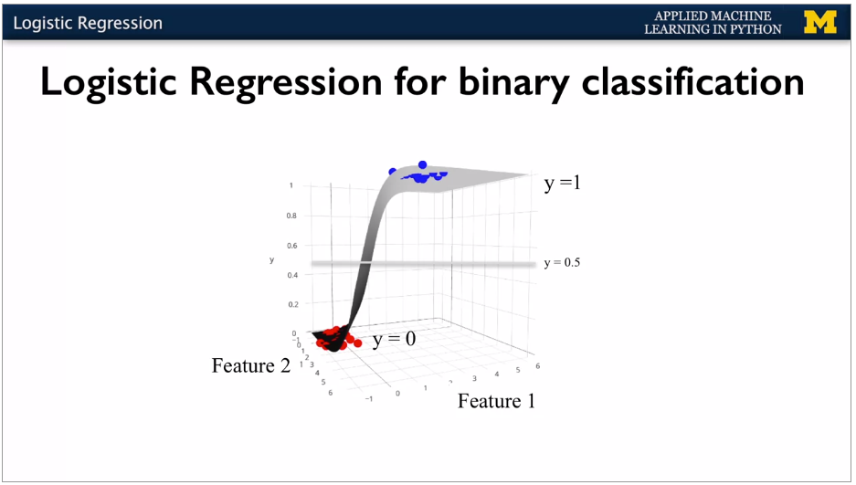
With 2 features, 3d view sort of looks like this.
 {width="4.489583333333333in"
height="2.5442300962379703in"}
 {width="4.489583333333333in"
height="2.5472145669291337in"}
 {width="4.40625in"
height="2.508721566054243in"}
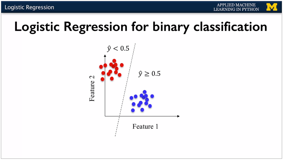
Output value is the probability of belonging to the class.
Regularisation (penalty for complexity) is on by default. Controlled with parameter C, defaults to 1. Higher C is less regularisation. Small C, tries to find coefficients closer to zero even if fit is worse. Power of regularisation only really visible with higher number of features.
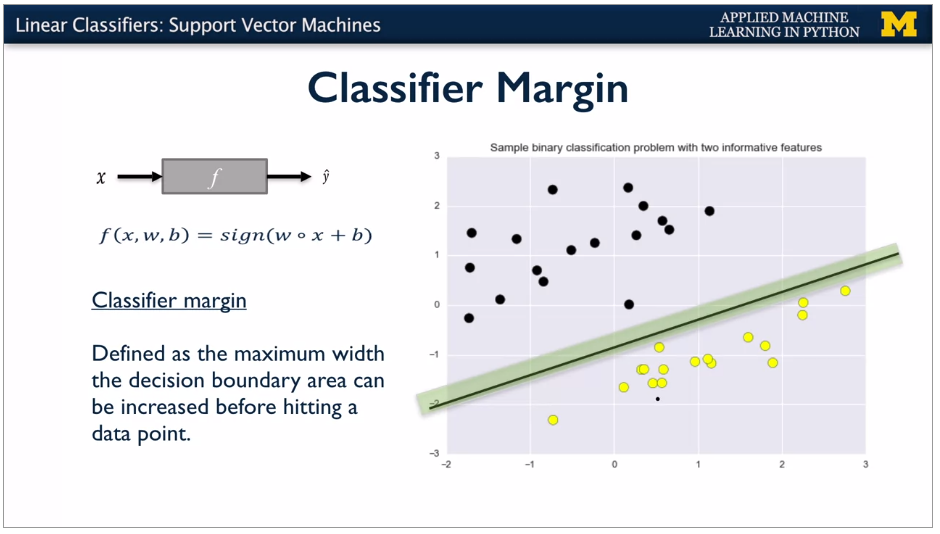
Take output of linear function and apply sign function to get +1 or -1.
Classier is good if get a broad decision boundary. Best is maximum margin. SVM can have linear or non linear model behind them. Kernel.
 {width="6.268055555555556in"
height="3.561111111111111in"}
 {width="6.268055555555556in"
height="3.561111111111111in"}
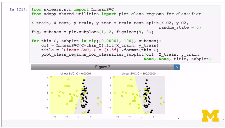
Trade off between wide decision boundary and misclassifying some points, controlled by Regularisation parameter C, set to 1 by default. Small C means more regularisation, so large decision boundary, even if more points are misclassified.
 {width="6.268055555555556in"
height="3.5347222222222223in"}
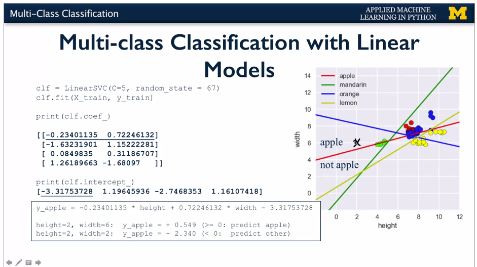
Real world is multi category output. Scikit learn converts to series of binary problems. Categorical items turned into binary for each class. 4 fruits -> 4 binary classifiers. Runs against each classifier in tern, and the highest one is the result.
 {width="6.268055555555556in"
height="3.517361111111111in"}
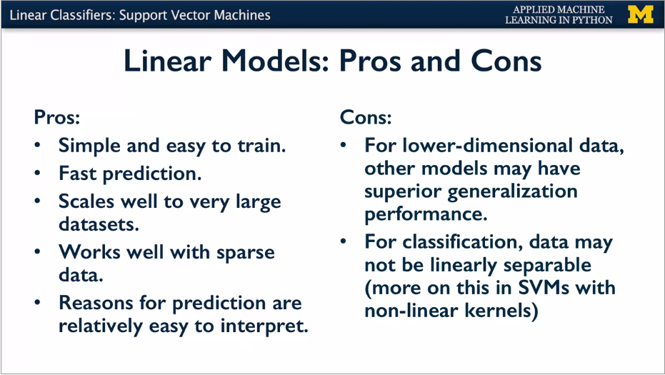
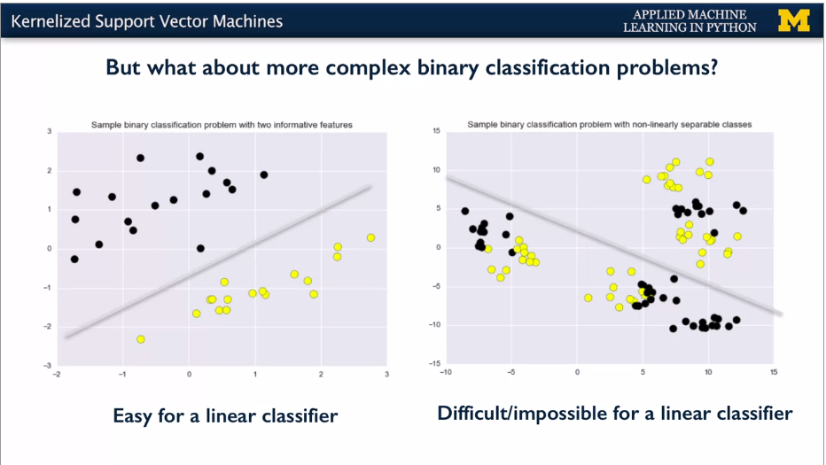
Linear SVM good for simple where close to linearly separable. E.g.
 {width="6.268055555555556in"
height="3.53125in"}
SVMs can do more complex classification and regression -- but this lecture is just classification.
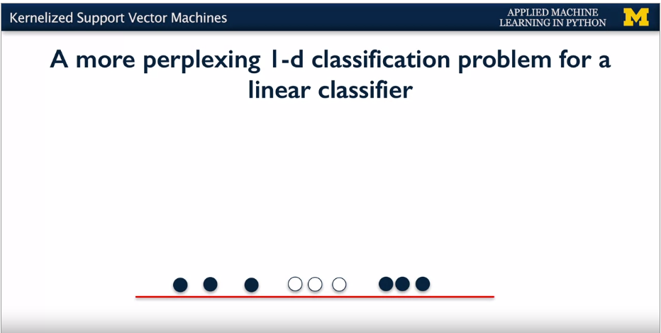
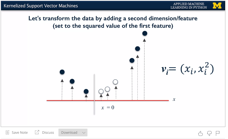
SVMs take feature space and transform to higher dimension space, and then use a linear classifier. Add e.g. a square feature. Bit like polynomial features to linear model.
 {width="6.268055555555556in"
height="3.154166666666667in"}
 {width="6.268055555555556in"
height="3.83125in"}
 {width="6.268055555555556in"
height="3.553472222222222in"}
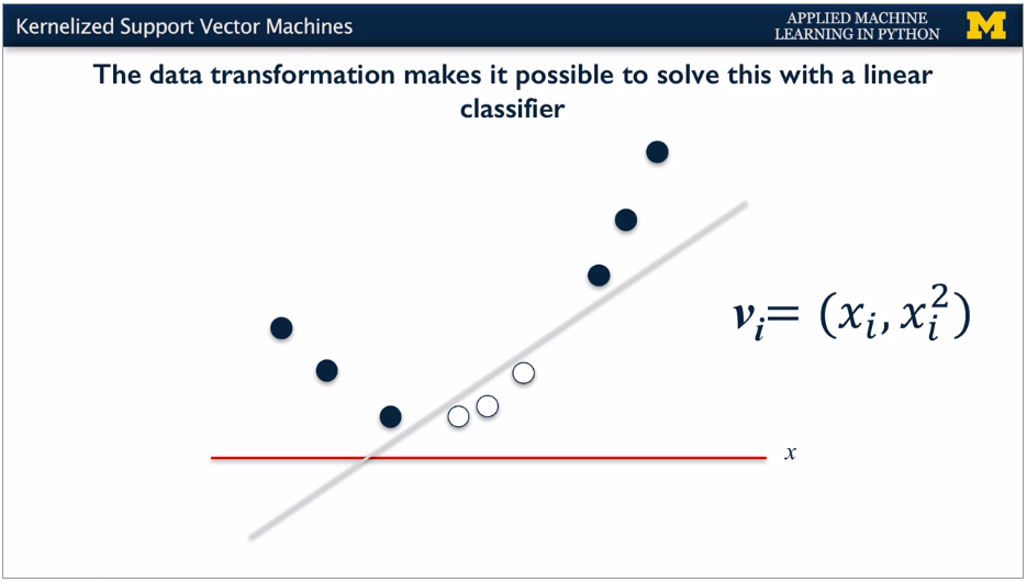
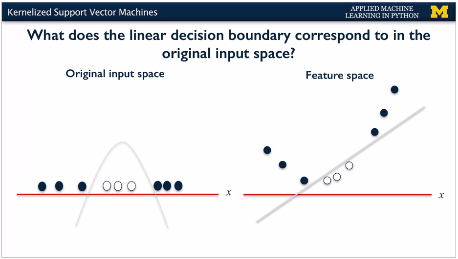
Linear classifier works well when have this extra dimension.
Create additional dimension and then use linear. When transform back to 1D, you get a parabolic decision boundary.
 {width="6.268055555555556in"
height="3.5520833333333335in"}
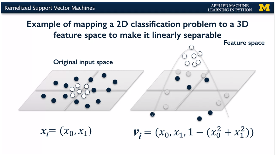
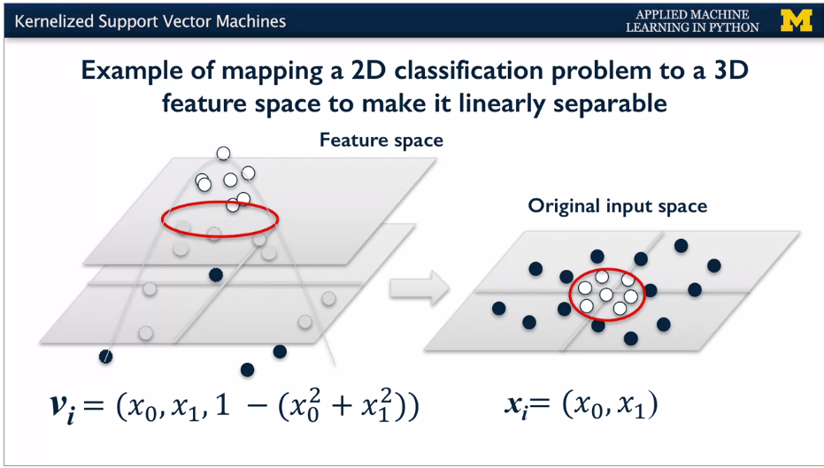
With more features: add 1 -- (x~0~^2^ + x~1~^2^)
 {width="6.268055555555556in"
height="3.573611111111111in"}
Moving back to original dimensions, get a parabola.
 {width="6.268055555555556in"
height="3.5618055555555554in"}
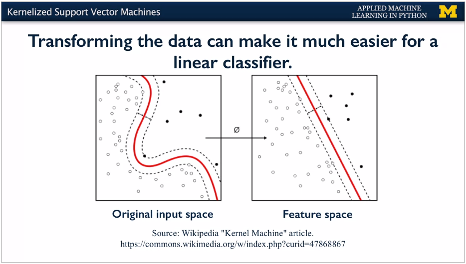
Several different possible transformations. E.g. RBF kernel, polynomial kernel.
 {width="6.268055555555556in"
height="3.5569444444444445in"}
 {width="6.268055555555556in"
height="3.5256944444444445in"}
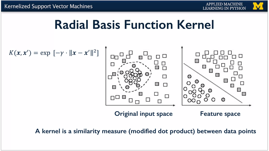
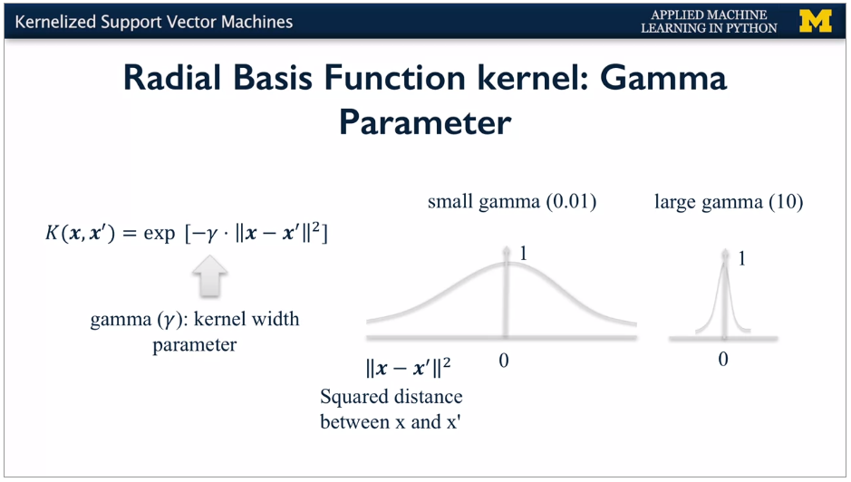
For the radial basis function kernel, the similarity between two points and the transformed feature space is an exponentially decaying function of the distance between the vectors and the original input space as shown by the formula here.
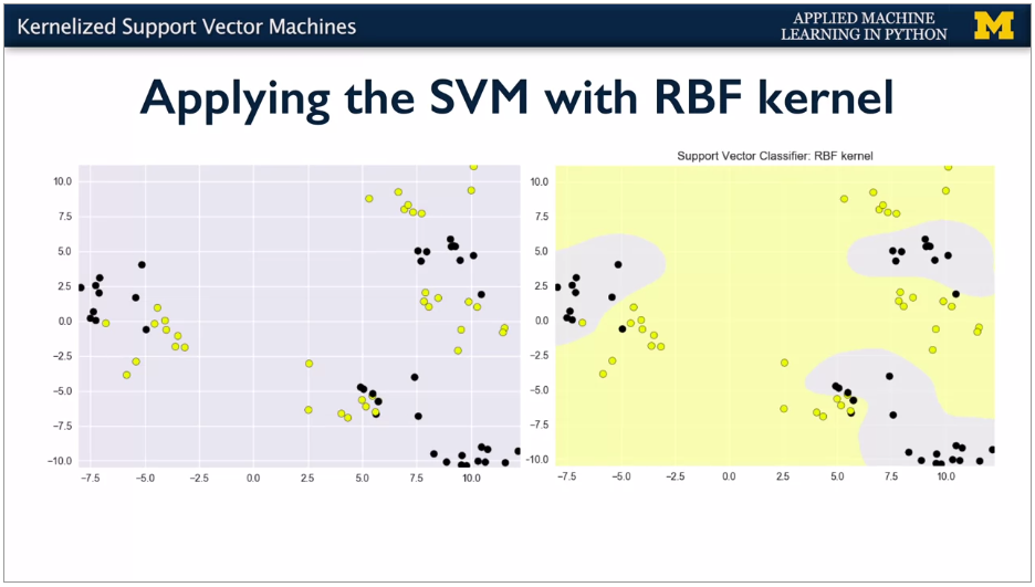
SVM makes the linear boundary with maximum margin in the transformed feature space. In the original space, it's curved.
Kernel Trick: internally doesn't need to really transform the data points. Just needs to do similarity calculations between points. So works OK for different data and many dimensions.
 {width="6.268055555555556in"
height="3.55625in"}
 {width="6.268055555555556in"
height="2.5194444444444444in"}
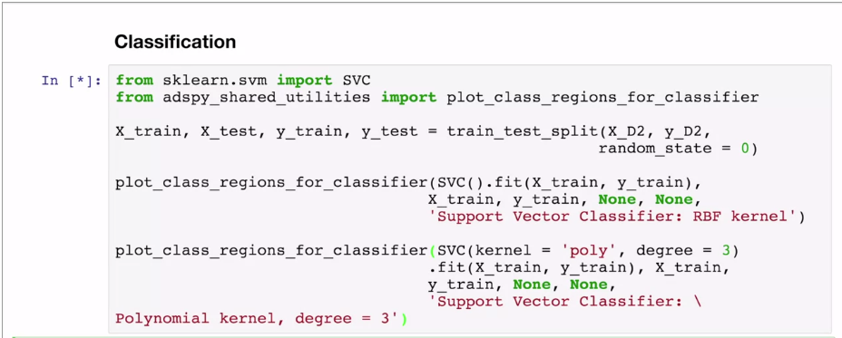
Polynomial kernel: different function. Takes degree parameter to affect complexity and cost.
RBF has parameter Gamma. Small gives larger similarity radius.
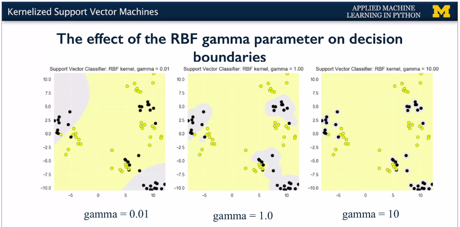
Small values of gamma give broader, smoother decision regions. While larger values of gamma give smaller, more complex decision regions.
You can set the gamma parameter when creating the SVC object to control the kernel width in this way, as shown in this code.
 {width="6.268055555555556in"
height="3.551388888888889in"}
 {width="6.268055555555556in"
height="3.0972222222222223in"}
You may have noticed that the RBF kernel has a parameter gamma.
Gamma controls how far the influence of a single trending example reaches, which in turn affects how tightly the decision boundaries end up surrounding points in the input space.
Small gamma means a larger similarity radius. So that points farther apart are considered similar. Which results in more points being group together and smoother decision boundaries.
On the other hand for larger values of gamma, the kernel value to K is more quickly and points have to be very close to be considered similar. This results in more complex, tightly constrained decision boundaries.You can see the effect of increasing gamma that is sharpening the kernel
in this example from the notebook.
Small values of gamma give broader, smoother decision regions. While larger values of gamma give smaller, more complex decision regions.You can set the gamma parameter when creating the SVC object to control the kernel width in this way, as shown in this code.
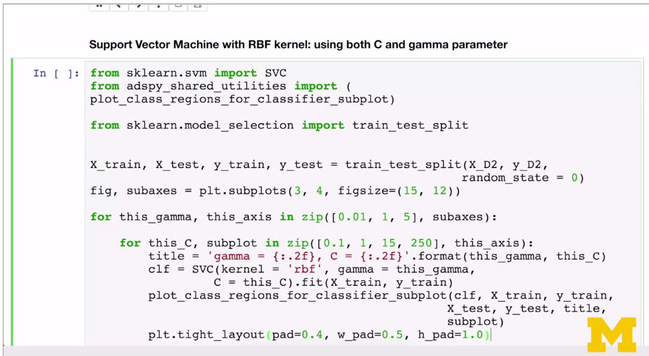
You may recall from linear SVMs that SVMs also have a regularization parameter, C, that controls the tradeoff between satisfying the maximum margin criterion to find the simple decision boundary, and avoiding misclassification errors on the training set. The C parameter is also an important one for kernelized SVMs, and it interacts with the gamma parameter.
This example from the notebook shows the effect of varying C and gamma together.
If gamma is large, then C will have little to no effect. Well, if gamma is small, the model is much more constrained and the effective C will be similar to how it would affect a linear classifier.
Typically, gamma and C are tuned together, with the optimal combination typically in an intermediate range of values. For example, gamma between 0.0001 and
10 and see between 0.1 and 100. Though the specifically optimal values will depend on your application.
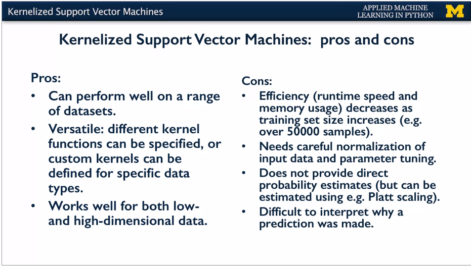
Kernelized SVMs are pretty sensitive to settings of gamma. The most important thing to remember when applying SVMs is that it's important to normalize the input data, so that all the features have comparable units that are on the same scale. We saw this earlier with some other learning methods like regularized regression.
 {width="6.268055555555556in"
height="3.4444444444444446in"}
 {width="6.268055555555556in"
height="3.548611111111111in"}
Kernel type defaults to RBF. Kernel has specific parameters, RBF very sensitive to gamma. C regularisation applies to all, typically tuned together with gamma.
Used to evaluate model, not tune.
Single train test split to get estimate for how well the model will genaralise to unseen data. Test set drawn from the same distribution as the training set.
Cross validation means multiple train test splits. Train test split gives different results based on initial seed. Cross validation gets rid of this.
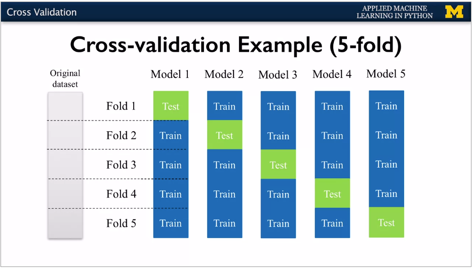
K-fold validation: e.g. 5 fold
 {width="6.268055555555556in"
height="3.55in"}
Get 5 accuracy values.
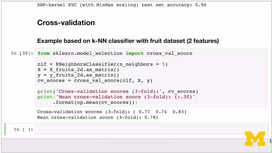
Use cross_val_score to implement.
 {width="6.268055555555556in"
height="3.5395833333333333in"}
Different accuracy values tell you how sensitive the model is to different training sets, understand range of performance.
 {width="6.268055555555556in"
height="3.553472222222222in"}
 {width="6.268055555555556in"
height="3.55in"}
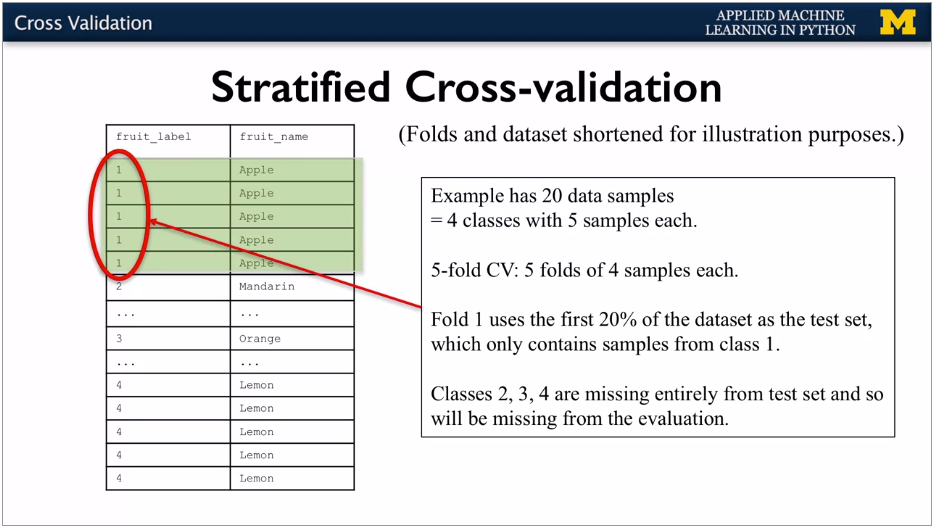
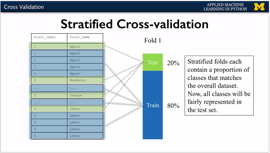
Scikit learn does stratified cross validation by default for classification. For regression, does standard.
Leave-one-out cross validation: test by leaving out just one sample for each training set.
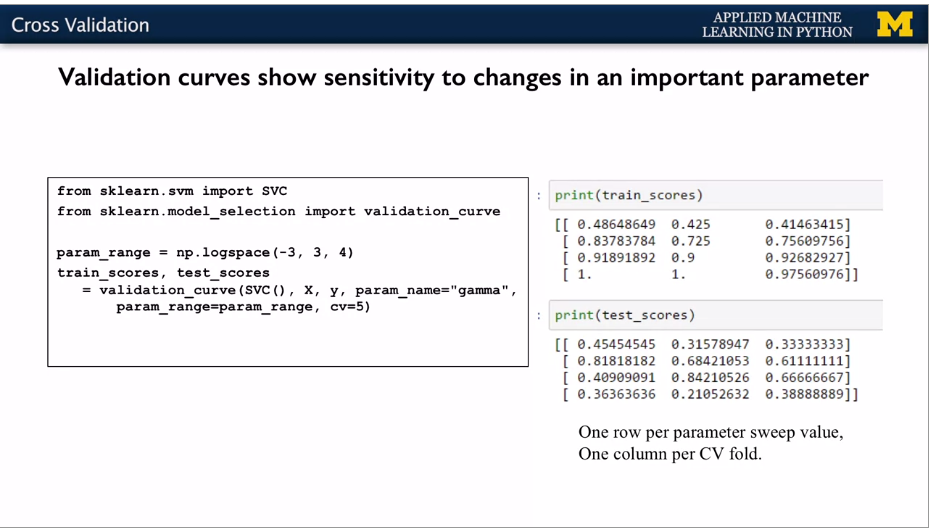 {width="6.268055555555556in"
height="3.55in"}
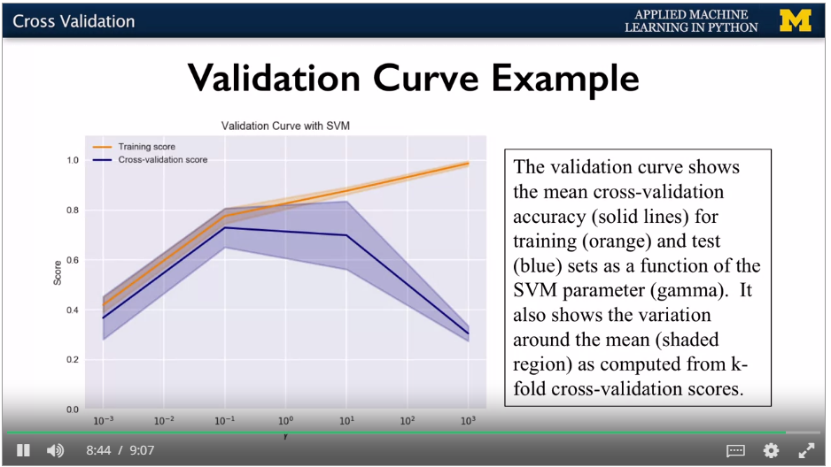 {width="6.268055555555556in"
height="3.5284722222222222in"}
Regression and classification
Good to find influential features in dataset.
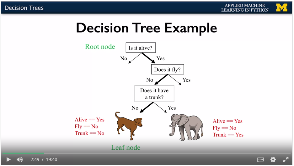
Have the most informative questions at the start.
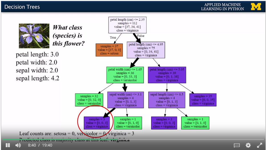
Root node at the top, leaf nodes at the bottom. Route determined by yes / no answers. Decision tree for predicting the class. Get to accurate classification quickly.
 {width="6.268055555555556in"
height="3.5520833333333335in"}
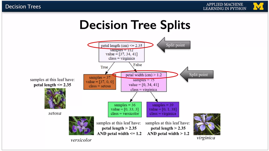
Iris, continuous values for features.
 {width="6.268055555555556in"
height="3.53125in"}
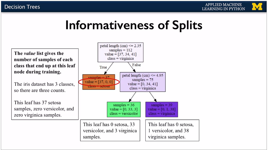
Each feature splits into 2 branches. Choose a split point for the value of the feature. Aim is to put the split at the point which gets the most information gain. If leaf is all one classification, then it's a pure node.
 {width="6.268055555555556in"
height="3.5256944444444445in"}
 {width="6.268055555555556in"
height="3.529861111111111in"}
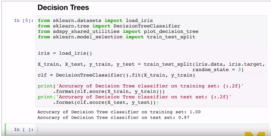
Can use for regression also.
 {width="6.268055555555556in"
height="3.14375in"}
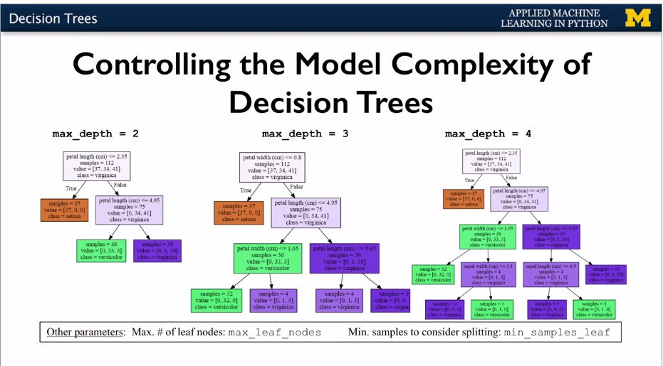
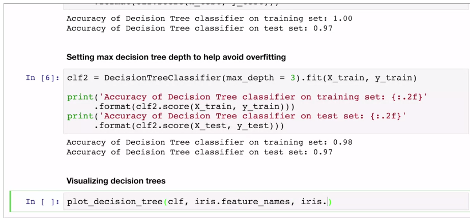
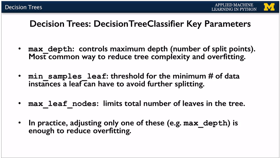
Overfitting control: can use pre-pruning with to stop the growth of complexity. Or post pruning: let it grow then prune back to simpler form. Scikit learn only does pre-pruning, using max_leaf_node, and max_depth. Plus Min_samples_leaf parameter.
 {width="6.268055555555556in"
height="3.467361111111111in"}
Visualizing decision tree:
 {width="6.268055555555556in"
height="2.9097222222222223in"}
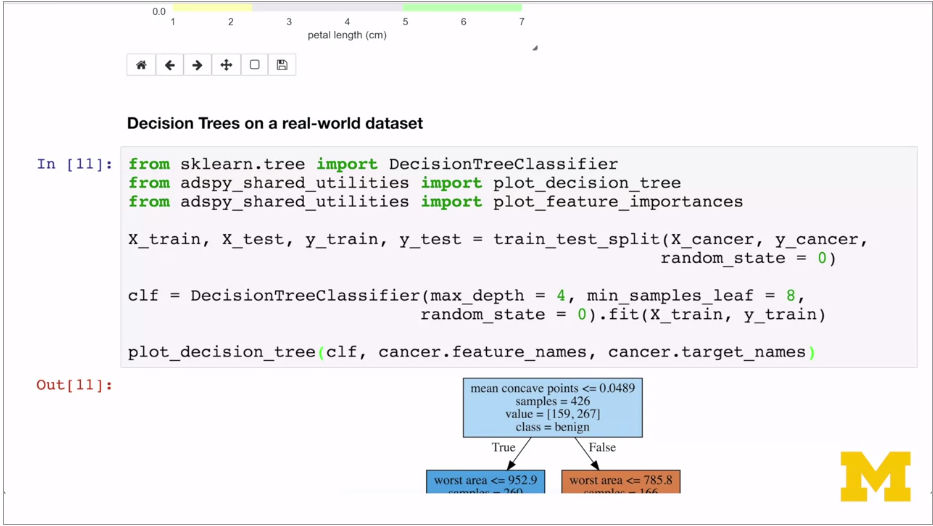
Plot_decision_tree is own function, Calls export graph vis function in scikit learn.
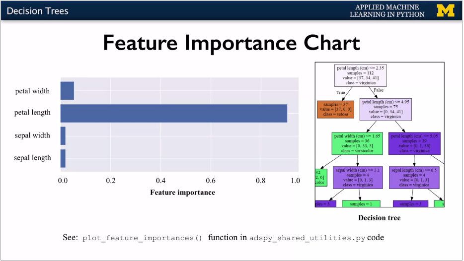
Useful to see the nodes being most informative. Feature importance calculation. How important is the feature to overall prediction accuracy. 0 means irrelevant, 1 means perfectly predicts. Numbers are normalised. Stored in feature_unimportances_
 {width="6.268055555555556in"
height="3.529861111111111in"}
 {width="6.268055555555556in"
height="3.5340277777777778in"}
 {width="6.268055555555556in"
height="3.5520833333333335in"}
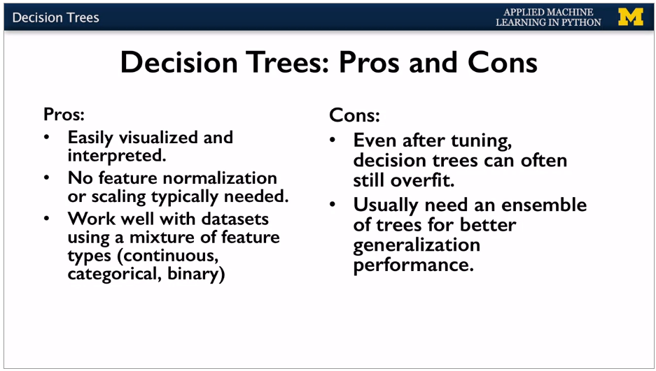
Good for initial feature selection. Can use without normalisiation as each feature runs independently. Good where different feature types (binary, continuous, categorical).
Key parameters. Generally adjusting one is enough.
 {width="6.268055555555556in"
height="3.529166666666667in"}
Domingos, P. (2012). A few useful things to know about machine learning. Communications of the ACM, 55(10), 78. doi:10.1145/2347736.2347755